Kafka Streams Concepts
Review of the streams concepts in Apache Kafka.
Kafka is a distributed, resilient, fault tolerant streaming platform that works with high data throughput. In this page, the main concepts of Kafka Streams technology will be covered.
- Data Streaming Concepts
- Kafka Streams Concepts
- Kafka Streams Architecture: Simple and Flexible
- Kafka Streams Compared to Other Tools
- How to Code Kafka Streams in Java?
- Handling Messages: KStreams and KTables
- Stateless and Statefull Operations
- Joins
- Use Cases and Examples
- References
Data Streaming Concepts
A Stream is an infinite sequence of messages. Pretty much everything can be seen as a stream of events: credit card transactions, stock trades, network packages to switches, etc. An inifinite and ever growing sequence of messages is also called an unbounded dataset. “Unbounded” because is a never-ending sequence of data. “Dataset” just because is a set of data.
In addition to this previous definition, there are other important characteristics in a stream model:
- Event Streams are Ordered: this is an important concept, because the order of things affects the end behavior (think about bank transactions of debit and credit).
- Data records are Immutable: this means that cannot be changed. When some transaction must be cancelled, actually a new transaction will be created to revert the action of the previous transaction. So, an ever-growing sequence of messages, indeed.
- Events are Replayable: a very important concept. This means that a particular sequence of messages can be executed again, in the same order, in a way that allows to understand errors, gather metrics and perform analysis.
Stream Processing Programming Paradigm
In this context, Stream Processing is the process of one or more event streams. It is a programming paradigm, such as batch processing and request-response.
- Request-Response: This is the lowest latency paradigm, with response times of few milliseconds - or less. It is usually blocking, so the client need to wait for the server to respond. In database terms, it is the same as OLTP (online transaction processing). This paradigm is often used by credit card transactions and time-tracking systems.
- Batch Processing: This is the highest latency/throughput option. The process is usually scheduled to run after midnight, and take a few hours to process a huge amount of data, generating stale information to be consumed by clients in the next day. The problem with this approach is that business evolved in a way that sometimes it is not acceptable to wait for the next day to get information.
- Streams Processing: This is a non-blocking option, that fills the gap between the blocking scenario of request-response paradigm and the timeframe of hours of processing, imposed by the batch processing paradigm. It is a more practical approach, since most business do not need to process data in milliseconds, but also cannot wait for an entire day to work with brand new data. This continuous, non-blocking processing attend a very broad range of use cases.
Stream Processing Concepts
Every data processing system has the ability to receive data, perform transformations, and save data elsewhere. Data streaming processing systems have some specific conceptions to consider in that scenario:
Time
It is a complex concept, that may be better covered when presented with some topics:
- Event Time: the time in which the record was created. The producer automatically add this information to the record when it is created, but sometimes you want to apply your own definition of event time, and it can be done simply by adding it as a field to the record.
- Log Append Time: the time that event arrive in the Kafka Broker. It is automatically added by Kafka Brokers in the moment that the message arrives (if Kafka was configured to do so), and is not that important to stream processing, actually, because it will make more sense to work with event time. But can be used in cases where the event time is not being produced.
- Processing Time: This is the time the message started to be processed. It is not reliable, because the processing can start days after the event was actually created. It can even differ from two threads in the same application. This is a notion of time that is better to avoid in practice.
It is also important to consider the concept of Time Zone: when working with time, it it important that all data is standartized to the same timezone, otherwise the results will be very hard to interpret and understand. If your scenario covers several timezones, it is important to define one as the standard and to adopt it consistently; often this means to store it and send in each message.
State
When dealing with a single message, the stream processing is very easy. But Streams start to became interesting when you have to handle multiple events, like counting the number of events per type, joining two streams to create a enriched stream of information, perform sum, averages, etc.
The information that can be collected between events is called State. There are two main types of states in the streaming paradigm:
- Internal State/Local State: state that is accessible to a specific instance of a single application. It is usually saved in an in-memory database. It is fast, but restricted to the amount of local available memory.
- External State: state that is saved in a external data store, usually a NoSQL database like Cassandra. It is good because the size is unlimited and data is available even to other systems. It is not so good because of the increased latency and complexity. Most stream processing apps try to avoid to handle with external systems, or at least to limit the usage, trying to cache information in internal states and to communicate to external states as rarely as possible.
Table/Stream Duality
Tables and Streams are complementary elements. Tables present the current state of something, while Streams present the events that cause this something to reach the current state. Sometimes we want one, sometimes other.
When a stream is converted to a table, it is said that the stream was materialized. And there are ways to get data changes from a database table (consider CDC) and import those to Kafka as a Stream of events that led to that end-state.
Windowed Operations
Most Stream operations should be considered in a slice of time (for instance, to process all events that happened last week). In that regard, the following window characteristics must also be considered:
- Window size: it is defined as unit of time. For instance, all events that happened in a 5-minute window.
- Advance Interval: It defines how often the window moves. It can be defined by specific period of time, or it can advance when there is a new event (a Sliding Window). For instance, if your window is 00:00-00:05 and the window advances at each two seconds, you may have the following windows after 4 seconds:
- 00:00-00:05
- 00:02-00:07
- 00:04-00:09
- and, in this case, all events that arrived with the event time of 00:03 will be part of windows 1 and 2 - but not 3.
- How long windows are updatable: For instance, if the window is defined as 00:00 to 00:05, and a record arrives at 00:10 with a event time of 00:02, it should or should not to be part of the window? If the window is updatable only until 00:07, for instance, this latest record will not be considered as part of the window - even if the event time is valid to that window.
If the advance interval is the same as the window size, it is called a Tumbling Window. If the windows overlap (the advance interval is less than the window size), it is called Hopping Window. If it is a Sliding Window, the window will move whenever there is a new record.
Windows can be aligned to a clock time (for instance, a 5 minute interval that moves every minute will have the first slice at 00:00-00:05 and the second slice at 01:00-06:00) or can be unaligned (and will start when application starts; the first slice can be 12:12-12:17 and the second slice will be 12:13-12:18).
Stream Processing Design Patterns
Some of the most common design patterns for stream processing are pointed below:
Single Event Processing
Treats events in isolation. For instance, a stream can read log records and, if a record has a ERROR message, send it to a particular error stream, and if not, send it to a regular stream. There is no need to save state, since there is no relation between messages.
Processing with Local State
This approach uses a local store to save state. For instance, if your requirement asks you to calculate the min and max value of a specific time window, you need to save state somehow, and you can adopt shared state or local state in order to accomplish it.
In this particular case, where we’re handling a group by aggregation, we can assume that all related messages are in the same partition of a same topic (because of the same key). So, according to the consumer group rules, each instance will get a particular partition to read data. So, in this case, we can use a local state, since a particular instance do not need to share with others, because it has a particular partition, exclusive to it.
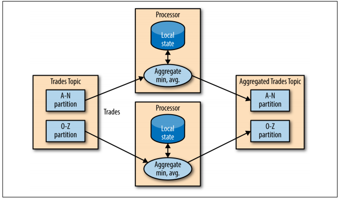
Figure: Local State - from “Kafka: The Definitive Guide” e-book.
When application starts to adopt local state, a more complicated scenario arises, and a new set of concerns must be considered:
- Memory usage: local state memory must fit into application’s available memory
- Persistence: data is saved in a memory using a RocksDB database. But all changes are also sent to a log-compacted Kafka topic. So, a state is not lost if Kafka application shuts down - in this case, the events can be reread from this Kafka topic.
- Rebalancing: Partitions can be reassigned for different consumers. In that case, the instance that loses partition must store the last good state, and the instance that receives this partition must recover the correct state. This will work because the state is in a Kafka topic, as said above.
Multiphase Processing/Repartitioning
The above approach works for group by types of aggregates. But what if the requirement is not specific to individual partitions, but to data obtained from all partitions? In that particular case, the approach is still simple: to perform local-state actions for particular partitions and them send this aggregated data to a second topic, with only one partition. So, a simple consumer can read this data to consolidate the overall results.
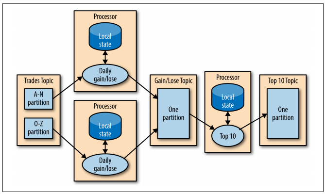
Figure: Multiphase Processing - from “Kafka: The Definitive Guide” e-book.
Processing with External Lookup: Stream-Table Join
Sometimes, stream processing requires access to an external source of data.
Let’s consider that we have to reach a database in order to process our stream. The basic approach would be to access database every time an event occur, enriching the data and sent it to another topic.
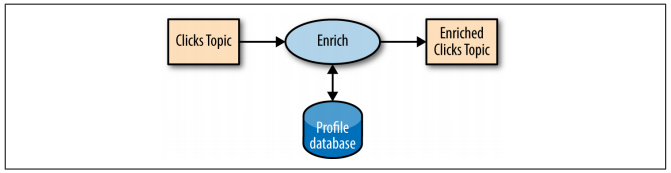
Figure: External Lookup - from “Kafka: The Definitive Guide” e-book.
But this is a dangerous approach, because adds network latency. In addition, stream processing systems can usually handle 100-500k events/sec, but database can only handle 10k events/sec in a very good scenario.
A better scenario would be to cache database in the streaming application. In order to make this cache to be as precise as possible, one could use Kafka Connector for CDC (database events that can be captured) and send this events to a topic.
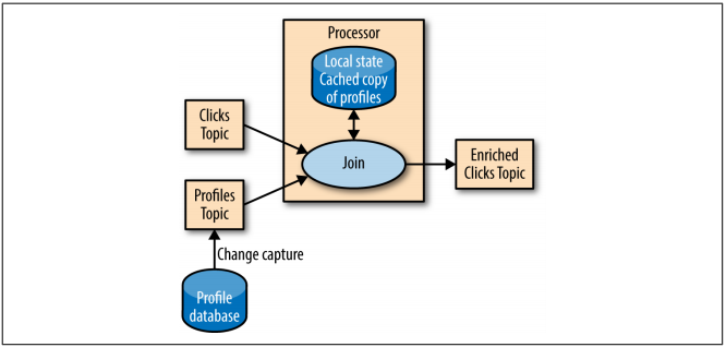
Figure: External Lookup - from “Kafka: The Definitive Guide” e-book.
Now, data can be looked up from local cache and the event can be enriched without the latency issues previously pointed.
This procedure is called a Stream-Table Join because one of the streams represents changes to a locally cached table.
Streaming Join
This is the scenario in which data from two different streams are joined. In order for this to be possible, it is necessary for both topics to have the same key.
Let’s consider a topic of user’s search queries, and another topic of user clicks. We can join these two topics in order to understand which search is more effective for users in terms of click results.
The two topics must be joined considering a time window. So, let’s say that the expected time from search to click is five seconds.
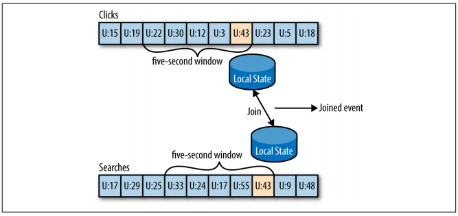
Figure: Streaming Join - from “Kafka: The Definitive Guide” e-book.
The keys are also used as join keys, to relate both streams. So, in a given window (U:43, in the figure), is guaranteed that both search and click events for a particular user will exist for the same partition (for instance, partition 5) of both topics. This join-window for both topics is saved in the local RocksDB cache, and this is how it can perform the join.
Out-of-Sequence Events
This is the case in which events arrive late in the stream, for instance, due to network connectivity issues.
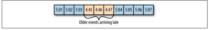
Figure: Out of Sequence Events - from “Kafka: The Definitive Guide” e-book.
Kafka Streams is able to recogzine that an event is out of sequence (check if the event time is older that the current time), define a time period to accept and reconcile out-of-sequence events, and to update this events.
This is typically done by maintaining multiple open aggregated windows in the local state, giving the developers the ability to configure how long these windows are available for updates. The longer this local state windows remain opened, more memory is required to maintain it.
Kafka Streams always writes aggreegation result in log-compacted result topics ( only the latest state is preserved).
Reprocessing
In some cases, we can change our streaming application (for both new features ou bug fixes). Hence, there is a need to run this new app version on the same event stream of the old application, generating new stream of events.
The good practice here is just to use a new consumer group for this new app, to start reading from the first offset of the input topic, generating a new output topic. Then, both old and new output topics can be compared.
Use Cases and Scenarios for Streaming
As previously said, stream processing is useful in scenarios where you cannot wait for hours to complete (as batch), but still you don’t have to get the return of processing in milisseconds (as request-response).
Some cases that will fit in this scenario (extracted from the “Kafka Definitive Guide” e-book) are below:
-
Customer Service in Hotel: considering an online hotel reservation, it is not acceptable to wait for an entire day (as batch) to have the confirmation. Instead, it is expected (as near real time) to have, in minutes, the confirmation sent by email, the credit card charged on time, and additional information of customer history appended to the reservation, for additional analysis.
-
Internet of Things: In stream processing, it is a common scenario to try to predict when maintenance is required, by reading sensor information from devices.
Choosing a Stream Processing Approach for Your Application
Depending of the nature of the application, approaches for stream processing may differ. It is important to choose the best solution for your application based on its particular characteristics.
Different types of applications are listed below:
- Ingest: the goal is to get data from one system and send to another, with some minor modifications to comply with target system expectations. For instance, some simple ETL mechanisms.
- In that case, a Kafka Connect may suffice (since it is a ingest-focused system).
- But if there is some level of transformation, Kafka Streams can be a good choice, but you need to make sure that Connectors for Source and Sink are also good enough.
- Low latency actions: applications that require very fast response. For instance, some detection fraud systems.
- Request-response patterns are better to suit this particular need.
- But if streams is still the choice, one must make sure that the model is based on event-by-event low latency, instead of microbatching
- Asynchronous microservices: microservices that perform simple actions on behalf of a larger business process, such as updating a database. It may need to maintain a local cache events as a way to improve performance.
- A stream processing system must be able to integrating with Kafka, must have ability to deliver content to microservices local caches, and good support for a local store that serves as a cache or materialized view of the microservice data
- Near real time data analytics: where complex aggregations and joins are required in order to produce relevant data.
- It is expected a stream processing mechanism with great local store support, in order to perform the complex aggregations, joins, and windows.
Kafka Streams Concepts
Kafka Topic is an example of Stream: it is replayed, fault-tolerant and can be ordered.
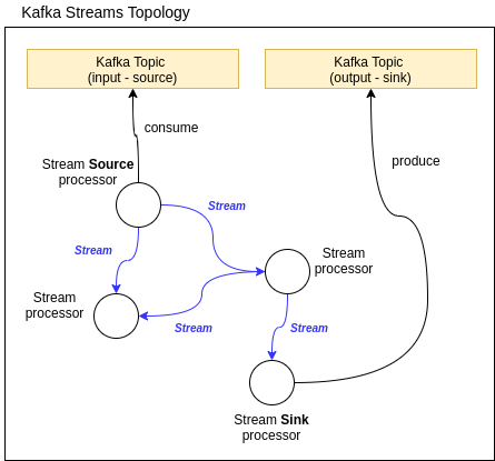
Streams work in a Topology concept. Stream Processor is a node on that Topology, responsible to process the stream in a specific way. It can create new streams, but never change an existing stream - since it’s immutable. Stream Processors are connected by Streams.
Figure: Kafka Streams Topology.
A Source Stream Processor is the one who connects to a topic to bring data to the topology.
- It has no parent in the topology
- Do not transform data
A Sink Stream Processor is the one who send processed data back to a Kafka topic.
- It is a leaf in the topology; has no successors
- Do not transform data
So, as we can see, Kafka Streams only iteracts to Kafka Topics, to get and send data. This is different than Kafka Connect, that brings and send data to all kinds of different external systems.
Kafka Streams Architecture: Simple and Flexible
Kafka Streams are very simple in terms of architecture. A Kafka Streams application is just a standard java application (jar) that runs in a JVM as an isolated process. The concept of “cluster” do not apply to it.
Since Kafka Streams inherits Kafka characteristics, it also can be considered fault-tolerant and scalable.
Because of this simple architecture, it supports any application size - from the smallest to the largest one.
Where is Kafka Streams in a Overall Kafka Architecture?
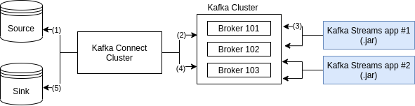
Figure: Kafka Streams Overview.
The numbered steps are below described:
- Kafka Source Connector gets some data
- Kafka Source Connector ask to its Worker to send data to the Broker’s topic
- Kafka Streams gets data from the Broker’s topic, processes it and send it back to another topic
- Kafka Sink Connector asks to its Worker to get data from the second topic
- Kafka Sink Connector send processed data to the destination
True Streaming: One Record at a Time
Kafka Streams process one record at a time. It is not a batch mechanism, like Spark, but a stream mechanism that process and transform records, one at a time.
Exactly Once Capabilities
Kafka Streams supports exactly once capabilities. This means that each message will take the read-process-write operation only one time. It is guaranteed that no input message will be missed or no duplication will be produced.
It can be guaranteed because both input and output systems are Kafka.
Common Problems Without Exactly Once
Lets consider the following flow of events:
- 1) Kafka Streams app get message from Broker (input topic)
- 2) Kafka Streams app send processed message back to Broker (output topic)
- 3) Kafka Streams app get ack from the Broker (output topic)
- 4) Kafka Streams app commit offsets related to the output topic
If the step 3 do not occur (messages are being processed but not confirmed to the clients), the retry mechanism will make clients to send the messages again. Kafka Broker will get duplicated messages.
If the step 4 do not occur (data is saved in the output topic and ack’ed by the clients, but the offset was not commited), other clients will consume the same messages again (because they will read from the offset, which was not updated).
Offsets are commited from time to time - this is not an atomic operation - and, in the meanwhile, network issues (for instance) can prevent this commit to happen
There are cases where is acceptable to have duplicates (like page stats, or logs). But in scenarios where precision is a requirements (financial business, for instance), the Exacly Once semantics is usually mandatory.
Solving those problems with Exactly Once
Kafka consumers and producers can use the concept of idempotency. So, duplicated messages are always identified and discarded.
In an advanced Kafka Streams API, it is possible to write messages in different topics as a parte of a big transaction and only commit it if data is saved in all topics.
In order to adopt exactly semantics in Kafka Streams, one must add the following property:
import org.apache.kafka.streams.StreamsConfig;

// StreamsConfig.PROCESSING_GUARANTEE_CONFIG="processing.guarantee"
// StreamsConfig.EXACTLY_ONCE="exactly_once"
properties.put(StreamsConfig.PROCESSING_GUARANTEE_CONFIG,
  StreamsConfig.EXACTLY_ONCE);
How Exactly Once is supported in Kafka Streams?
Kafka Streams internally adopts Transaction API to make sure that data is saved in a way that can’t be lost:
- acked data: sent to sink topics
- state update: sent to a changelog
- offset commit: sent to a offset topic
Data is saved (or not) atomically in the three topics above mentioned. So, the scenarios of duplicate writer and duplicate processing do not occur.
Theses three steps are very hard to get in a stream processing technology, but Kafka can handles them properly.
More Information
More details related to Exactly Once capabilities can be found in the three articles below:
- Exactly-Once Semantics Are Possible: Here’s How Kafka Does It (06/2017): Explain the basics of Exacly Once semantics, and how Kafka was able to handle it in version 0.11.
- Transactions in Apache Kafka (11/2017): Explain how Kafka Transaction API works
- Enabling Exactly-Once in Kafka Streams (12/2017): Explain how Kafka Streams make use of Transaction API to support Exacly Once capabilities
Kafka Streams Internal Topics
Some intermediate topics are created internally by Kafka Streams:
- Repartitioning Topics: to handle stream key transformation
- Changelog Topics: to handle aggregations of messages
Messages in those topics will be saved in a compacted way. Those topics have the prefix application.id, and are basically used to save/restore state and to partition data.
These internal topics are managed exclusively by Kafka Streams, and must never be directly manipulated.
Scaling Kafka Streams Application
Kafka Streams uses Kafka Consumer, so the same rules apply.
- Each partition can only be read by a Kafka Stream App Process (for the same consumer group) at a time
- If you run more Kafka Stream processes than the number of partitions, those aditional processes will remain inactive
So, for each partition to be consumed in a topic, it could have a Kafka Streams application process running. For instance, if a topic has 3 partitions, so three Kafka Stream Application processes could be run in parallel to read data from the topic.
There is no need for any cluster! Just run the Java process and that’s it.
Kafka Streams also handle rebalancing (in a case that one of the Kafka Streams application processes dies), just as with consumers.
Streams Repartition
Each operation that changes the key (Map, FlatMap and SelectKey) triggers repartition. Once a Stream is marked to be repartitioned, it only actually applies it when there is a real need (for instance, when a .count() method is called).
Repartition is a Kafka Streams internal operation that performs some read/write to Kafka Cluster, so there is a performance penalty.
- A topic with “_repartition” suffix is created in Kafka to handle repartitions
It is a good idea to only use the APIs that trigger repartition if there is a actual need for key changing; and, otherwise, to adopt their value conterparts (MapValues and FlatMapValues).
KTables and Log Compaction
Log Compaction is topic attribute that improves performance (meaning less I/O and less reads to get to the final state of a keyed data).
It can be used in cases where only the latest value for a given key is required. Since this is the exactly situation of a KTable, it is right to assume that each topic that uses KTable would be set as log-compacted.
KTable insert, update or delete records based on key value, so old records with the same key will be discarded.
Kafka Streams Compared to Other Tools
This table is a comparison between Kafka Stream and another tools the perform similar job (Spart Streaming, Apache NiFi and Apache Flink):
| Item | Kafka Streams | Other Related Tools |
|---|---|---|
| Mechanism | Stream | Micro Batch |
| Requires Cluster? | No | Yes |
| Scale just by adding Java Processes? | Yes | No |
| Exactly Once Semantics related to Kafka Brokers? | Yes | No (at least once) |
| Based on code? | Yes | Yes=Spark Streaming and Flink; No=NiFi (drag and drop) |
How to Code Kafka Streams in Java?
There are two main ways:
- High Level (DSL): a more practical approach
- Low Level Processor API: a more detailed approach. It may be used to write something more complex, but usually it is not necessary to adopt it.
Kafka Streams Application Properties
Kafka Streams runs over Kafka Consumer and Kafka Producer, so it also uses their properties. In addition, it defines your own set of properties:
application.id: this property is for Kafka Streams only. It must have the same value of group id of the consumer. It is defined by the constantorg.apache.kafka.streams.StreamsConfig.APPLICATION_ID_CONFIG.bootstrap.server: same as Kafka. It is defined by the constantorg.apache.kafka.streams.StreamsConfig.BOOTSTRAP_SERVERS_CONFIG.auto.offset.reset: This is a consumer property. use earliest (to consume topic from the beginning) or latest. It is defined by the constantorg.apache.kafka.clients.consumer.ConsumerConfig.AUTO_OFFSET_RESET_CONFIG.processing.guarantee: Use exactly_once here, for obvious behavior. It is defined by the constantorg.apache.kafka.streams.StreamsConfig.StreamsConfig.PROCESSING_GUARANTEE_CONFIG.default.key.serde: This is used for key serialization and deserialization. It is defined by the constantorg.apache.kafka.streams.StreamsConfig.DEFAULT_KEY_SERDE_CLASS_CONFIG. For instance, it can assume the valueorg.apache.kafka.common.serialization.Serdes.StringSerde(default)default.value.serde: This is used for value serialization and deserialization. It is defined by the constantorg.apache.kafka.streams.StreamsConfig.DEFAULT_KEY_SERDE_CLASS_CONFIG. For instance, it can assume the valueorg.apache.kafka.common.serialization.Serdes.StringSerde(default)
Running as a JAR
Kafka Streams should be deployed as a fat jar (containing the code and its dependencies), that can be created using a maven assembly plugin. The jar articact must have a main method in order to run properly.
Handling Messages: KStreams and KTables
A Kafka Stream can be handled as a KStream or KTable.
KStream
In a KStream, all data is INSERTED. It is similar to the log concept (data are inserted in sequence). There is no end, so it have infinite size (always wait for new messages to arrive).
The following table describes the representation of a topic using KStream:
| Topic (key, value) | KStream |
|---|---|
| (alice, 18) | (alice, 18) |
| (bob, 22) | (alice, 18) |
| (bob, 22) | |
| (alice, 19) | (alice, 18) |
| (bob, 22) | |
| (alice, 19) |
As we can see, data is always appended to the end of a KStream, and there is no relation between old and new data.
KTable
KTable behaves more like a table. It is similar to the concept of log compacted topics. UPDATE is performed in non-null values, and DELETE occurs in messages with null values.
The following table describes the representation of a topic using KTable:
| Topic (key, value) | KTable |
|---|---|
| (alice, 18) | (alice, 18) |
| (bob, 22) | (alice, 18) |
| (bob, 22) | |
| (alice, 19) | (alice, 19) |
| (bob, 22) | |
| (bob, null) | (alice, 19) |
As we can see, data with a new key was inserted, data with the same key was updated, and data with null value was deleted.
KStream x KTable Usage
KStream should be used when:
- data is read from non-compacted topic
- if a new data is parcial and transactional
KTable should be used when:
- data is read from log compacted topic
- if a database-like structure is required (each update is self-sufficient)
Read/Write Operations
Reading Data
Data can be read from a Topic in Kafka Streams using KTable, KStream or GlobalKTable. The API is very similar, as presented below:
KStream<String, Long> wordCounts = builder.stream(Serdes.String(), Serder.Long(), "some-topic");KTable<String, Long> wordCounts = builder.table(Serdes.String(), Serder.Long(), "some-topic");GlobalKTable<String, Long> wordCounts = builder.globalTable(Serdes.String(), Serder.Long(), "some-topic");
Writing Data
Each KStream or KTable can be write back to Kafka topics.
When using KTable, consider log compacted mode in your related topic, so it can reduce disk usage
Some operations related to data writing:
TO:is a terminal, sink operation, used to write data in a topic.stream.to("output-topic");table.to("output-topic");
THROUGH:it writes data to a topic and gets a stream/table of the same topic. So, it is not a terminal operation.KStream<String, Long> newStream = stream.through("output-topic");KTable<String, Long> newTable = table.through("output-topic");
The KStream/KTable Duality
Streams and tables are the same, but represented differently. So, they can be related in particular ways.
Stream as Table
A KStream can be seen as a KTable changelog, where each record in a stream captures a state change in a table.
Table as Stream
A table can be considered a snapshot, in a given period of time, of the latest value for each key
Transformation: KTable to KStream
KTable<String, Long> table = ...
KStream<String, Long> stream = table.toStream();
Transformation: KStream to KTable
First option: call an aggregated operation in the KStream; the result will always be a KTable.
KStream<String, Long> stream = ...
KStream<String, Long> table = stream.groupByKey().count();
Second option: Write a KStream in Kafka and read it later as a KTable
KStream<String, Long> stream = ...
stream.to("some-topic");
KStream<String, Long> table = builder.table("some-topic");
In this case, it will read each record and perform based on the key and value characteristics:
- if the key do not exists, the record will be inserted into the KTable
- if the key already exists and the value is non-null, the record will be updated
- if the key already exists and the value is null, the record will be deleted
Stateless and Statefull Operations
Stateless operations are those who do not require knowledge of previous operations.
Statefull operations are those who depends on previous operations - for instance, to count messages based on aggregation rules considering previous data.
Stateless Operations
Select Key
This operation sets a new Key for a record. Record is marked for repartition (since key was changed).
// (null, "alice") -> ("alice", "alice")
rekeyed = stream.selectKey((k,v) -> v);
Map / MapValues
Gets one record and returns one record (1 to 1 transformation).
| Map | MapValues |
|---|---|
| Applied to Keys and Values | Applied only to Values |
| Alter keys (trigger repartition) | Do not alter keys |
| Only for KStreams | For KStreams and KTables |
// (alice, "Java") -> ("alice", "JAVA")
uppercase = stream.mapValues(value -> value.toUpperCase());
Filter / FilterNot
Gets one record and returns zero or one record. A FilterNot is just the logical inverse of a Filter.
Filter characteristics:
- Do not change keys and values
- Do not trigger repartition
- It can be used in KStream and KTable
// ("alice", 1) -> ("alice", 1)
// ("alice", -1) -> record is discarded
KStream<String, Long> positives = stream.filter((k, v) -> v >= 0);
FlatMap / FlatMapValues
Gets one record and returns zero, one or more than one records (an iterable).
| FlatMap | FlatMapValues |
|---|---|
| Change Keys | Do not change keys |
| Trigger repartition | Do not trigger repartition |
| Only for KStreams | Only for KStreams |
// ("alice", "I like coffee") -> ("alice", "I"), ("alice", "like"), ("alice", "coffee")
aliceWords = aliceSentence.flatMapValues(v -> Arrays.asList(v.split("\\s+")));
Branch
Branch is a very interesting concept. It splits a KStream based on particular predicates.
- Predicates are evaluated in order. The first to match gets the record
- Records only goes to single, unique branch
- If a record makes no match with any of the predicates, it is discarded
Consider the following branch structure:
KStream<String, Long>[] branches = stream.branch(
  (k, v) -> v > 100,  // first predicate
  (k, v) -> v > 10,   // second predicate
  (k, v) -> v > 0     // third predicate
);
| Data Stream | branches[0] (v>100) | branches[1] (v>10) | branches[2] (v>0) |
|---|---|---|---|
| (alice, 1) | (alice, 300) | (alice, 30) | (alice, 1) |
| (alice, 30) | (alice, 60) | (alice, 8) | |
| (alice, 300) | |||
| (alice, 8) | |||
| (alice, -100) | |||
| (alice, 60) |
The record (alice, -100) was discarded from the Stream, since it do not match any of the three predicates. The other records were related to specific branches based on the branch predicates. The order of predicates change the result, so define the proper order of branch predicates is very important.
Peek
The peek method allow us to run an action that do not generates collateral side effects in the stream (such as print data or collect stats) and then to return the same stream for further processing.
KStream<byte[], String> unmodifiedStream = stream.peek(
  (k, v) -> System.out.println("Key=" + key + "; value=" + value));
Stateful Operations
GroupBy (KTable)
This is required to work with aggregations. It triggers repartition, because key changes as a result of an aggregation.
// KTable groupBy method returns KGroupedTable
KGroupedTable<String, Integer> groupedTable = table.groupBy(
  (k, v) -> KeyValue.pair(v, v.length()), Serdes.String(), Serdes.Integer());

// KStream groupBy method returns KGroupedStream
KGroupedStream<String, Integer> groupedStream = stream.groupBy(
  (k, v) -> KeyValue.pair(v, v.length()), Serdes.String(), Serdes.Integer());
KGroupedTable / KGroupedStream objects
The aggregation methods (count, reduce and aggregate) can only be called in KGroupedTable or KGroupedStream objects. And these type of objects are obtained only by the return of groupBy and groupByKey methods (that can be called in both KStream and KTable, as above described).
So, ideally:
KGroupedStream gs = stream.groupBy(); gs.count() => XKGroupedTable gt = table.groupByKey(); gt.count() => N
All of the aggregation methods (count, reduce and aggregate), called in both KGroupedTable or KGroupedStream objects, always return a KTable.
Considering group streams related to null data:
KGroupStream:- Records with null data (for both keys and values) are ignored
KGroupTable:- Records with null keys are ignored
- Records with null values are treated like “delete”
Count
It just count the amount of records in the group, according to the null rules previously explained.
Aggregate
In a KGroupStream:
- It requires a
initializer, anadder(which has a key, a new value and an aggregated value), aserdeand astate-store name.
KTable<String, Long> aggregatedStream = groupedStream.aggregate(
  () -> 0L,
  (aggKey, newValue, aggValue) -> aggValue + newValue,
  Serdes.Long(),
  "aggregated-stream-store");
In the snippet above, aggKey type must match aggregatedStream key type (String), newValue must match aggregatedStream value (Long) and aggValue must match the initializer type (Long). The initializer and the new value can be different (translation will happen in the adder).
In a KGroupTable:
- It requires a
initializer, anadder(which has a key, a new value and an aggregated value), asubtractor(analogous behavior to the adder), aserdeand astate-store name.
KTable<String, Long> aggregatedStream = groupedStream.aggregate(
  () -> 0L,
  (aggKey, newValue, aggValue) -> aggValue + newValue,
  (aggKey, newValue, aggValue) -> aggValue - newValue,
  Serdes.Long(),
  "aggregated-stream-store");
The subtractor is used to treat the delete cases, previously explained.
Reduce
This is similar to aggregate, but the new and aggregated values must be of the same type (aggregate can deal with different types). It is much simpler: do not have both initializer and Serde.
It can work with just an adder:
KTable<String, Long> aggregatedStream = groupedStream.reduce(
  (aggValue, newValue) -> aggValue + newValue,    // adder
  "aggregated-stream-store");
Or can also be used with both adder and subtractor (to treat delete, as previously explained):
KTable<String, Long> aggregatedStream = groupedStream.reduce(
  (aggValue, newValue) -> aggValue + newValue,    // adder
  (aggValue, newValue) -> aggValue - newValue,    // subtractor
  "aggregated-stream-store");
KStream Transform/TransformValues
These applies a transformation in each record. It uses ProcessorAPI, which is less common.
- Transform: triggers repartition, since transformation occurs with both keys and values
- TransformValues: do not trigger repartition, since just transform values
Joins
A Join mechanism relates a KTable/KStream with another, creating another stream as part of it.
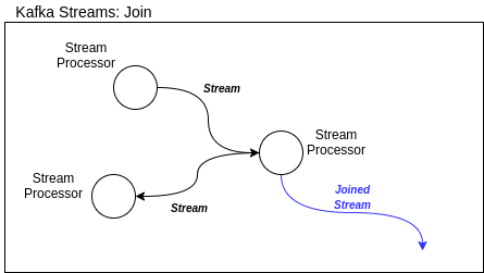
Figure: Kafka Streams Join.
There are three types of Join:
- Inner Join: like in database
- Left Join: like in database
- Outer Join: Left and Right combined
These types of joins are related to types of Streams, as described in the following table:
| Join Operand | Type | Inner Join | Left Join | Outer Join |
|---|---|---|---|---|
| KStream to KStream | Windowed | Supported | Supported | Supported |
| KTable to KTable | Non Windowed | Supported | Supported | Supported |
| KStream to KTable | Non Windowed | Supported | Supported | Not Supported |
| KStream to GlobalKTable | Non Windowed | Supported | Supported | Not Supported |
| KTable to GlobalKTable | N/A | Not Supported | Not Supported | Not Supported |
Joins constraints
- Joins can only occcur if data is co-partitioned (data came from different topics with the same number of partitions)
- GlobalKTable do not demand co-partitioning
- That is because data stays in every instance of the application, in memory and in the store
- However, the disk usage is a drawback for these application - but it is acceptable for a small amount of data
- GlobalKTable exists only as a DSL option (not in Processor API)
Use Cases and Examples
WordCount Demo and Topology
Kafka has a built-in demo class that allows us to test Kafka Streams. In order to test it, the following steps must be followed:
- Create topics for input and output with a specific name
$ ./bin/kafka-topics.sh --bootstrap-server localhost:9092 --create --topic \
    streams-plaintext-input --partitions 1 --replication-factor 1

$ ./bin/kafka-topics.sh --bootstrap-server localhost:9092 --create --topic \
    streams-wordcount-output --partitions 1 --replication-factor 1
- Send some data to the input topic
$ ./bin/kafka-console-producer.sh --broker-list localhost:9092 \
    --topic streams-plaintext-input

> java
> is
> pretty
> yes
> you
> are
> java
- Create a consumer to listen to the output topic
$ ./bin/kafka-console-consumer.sh --bootstrap-server localhost:9092 --topic \
    streams-wordcount-output --from-beginning --formatter \
    kafka.tools.DefaultMessageFormatter --property print.key=true --property \
    print.value=true --property \
    key.deserializer=org.apache.kafka.common.serialization.StringDeserializer \
    --property \
    value.deserializer=org.apache.kafka.common.serialization.LongDeserializer
- And now, run the built-in demo Kafka Streams class:
$ ./bin/kafka-run-class.sh \
    org.apache.kafka.streams.examples.wordcount.WordCountDemo
You should see the following:
> java    1
> is      1
> pretty  1
> yes     1
> you     1
> are     1
> java    2
Since it is a Stream, the word “java” will appear duplicated in the end, with a count of 2.
In terms of topology, the idea here is to perform an aggregation of records and grouping them, so they can be counted by the amount of duplicated words:
- Stream to create a stream:
<null, "Java pretty Java"> - MapValues to lowercase:
<null, "java pretty java"> - FlatMapValue split by space:
<null, "java">,<null, "pretty">,<null, "java"> - SelectKey to apply a key:
<"java", "java">,<"pretty", "pretty">,<"java", "java"> - GroupByKey before aggregation: (
<"java", "java">), (<"pretty", "pretty">), (<"java", "java">) - Count ocurrencies in each group:
<"java", 2>,<"pretty", 1> - To in order to write processed data back to Kafka
Topology for ‘Favorite Color’ Problem
Let’s consider the following requirements to a hipotetical problem:
- Data must be received in a format: (userId, color)
- It must accept only red, green and blue colors
- It must count the total of favorite colors from all users at the end
- The user’s favorite color can change
What is the proper topology for this problem?
- Stream data
- SelectKey defined as userId
- MapValue per color (lowercase)
- Filter for acceptable colors only (“red”, “green” and “blue”)
- To topic with log compaction
- that is because we want to count the latest color for all users, so we want to remove duplicates for ech user, maintaining only the last state. By sending data to a log compacted topic, Kafka will make sure that this will occurr as expected
- KTable read log compacted data
- GroupBy colors
- the userId is not relevant anymore; grouping is being performed over the last color choose by each user; only colors should be counted, not users.
- Count grouped colors
- To final topic